Block Group-to-CCA Crosswalk — xwalk_blockgroup2cca • cmapgeo

This table contains a set of factors to apportion Census block group-level data among Chicago Community Areas (CCAs). Separate factors are provided for apportioning housing unit, household, and population attributes. All factors were determined by calculating the percentage of a block group's housing units, households and population that were located in each of its component blocks, according to the 2020 Decennial Census, and then assigning each block to a CCA (based on the location of the block's centroid point). Use xwalk_blockgroup2cca for data from the 2020 decennial census or the American Community Survey (ACS) from 2020 onward. For data from the 2010 decennial census or ACS from 2010 through 2019, use xwalk_blockgroup2cca_2010.

xwalk_blockgroup2cca

xwalk_blockgroup2cca_2010

Format

xwalk_blockgroup2cca is a tibble with 2185 rows and 6 variables:

geoid_blkgrp: Unique 12-digit block group ID, assigned by the Census Bureau. Corresponds to blockgroup_sf. Character.
cca_num: Numeric CCA ID, as assigned by the City of Chicago. Corresponds to cca_sf. Integer.
hu_pct: Proportion of the block group's housing units (occupied or vacant) located in the specified CCA. Multiply this by a block group-level measure of a housing attribute (e.g. vacant homes) to estimate the CCA's portion. Double.
hh_pct: Proportion of the block group's households (i.e. occupied housing units) living in the specified CCA. Multiply this by a block group-level measure of a household attribute (e.g. car-free households) to estimate the CCA's portion.Double.
pop_pct: Proportion of the block group's total population (including group quarters) living in the specified CCA. Multiply this by a block group-level measure of a population attribute (e.g. race/ethnicity) to estimate the CCA's portion. Double.
emp_pct: Proportion of the block group's total jobs located in the specified CCA. Multiply this by a block group-level measure of an employment attribute (e.g. retail jobs) to estimate the CCA's portion. Not available in xwalk_blockgroup2cca_2010. Double.

xwalk_blockgroup2cca_2010 is a tibble with 2180 rows and 5 variables (no emp_pct).

Details

Generally speaking, block group boundaries align neatly with CCA boundaries as they tend to follow similar features (e.g. rivers, major roads, rail lines) but there are cases where the jobs, population, households and/or housing units in a block group are split across multiple CCAs, or else are partially within the City of Chicago and partially outside of it. For that reason, it is not appropriate to use a one-to-one block group-to-CCA assignment to apportion Census data among CCAs, and this crosswalk should be used instead.

To use this crosswalk effectively, Census data should be joined to it (not vice versa, since block group IDs appear multiple times in this table). Once the data is joined, it should be multiplied by the appropriate factor (depending whether the data of interest is measured at the housing unit, household, person or job level), and then the result should be summed by CCA. If calculating rates, this should only be done after the counts have been summed to CCA. The resulting table can then be joined to cca_sf for mapping, if desired.

If your data is only available at the tract level, you can use xwalk_tract2cca for a tract-level allocation instead.

Examples

suppressPackageStartupMessages(library(dplyr))

# View the block groups with housing units split between multiple CCAs
filter(xwalk_blockgroup2cca, hu_pct < 1)
#> # A tibble: 33 × 6
#>    geoid_blkgrp cca_num  hu_pct  hh_pct pop_pct emp_pct
#>    <chr>          <int>   <dbl>   <dbl>   <dbl>   <dbl>
#>  1 170310619024       6 1       1        1      1      
#>  2 170310701012       7 1       1        1      1      
#>  3 170310814031      32 0       0        0      0.306  
#>  4 170311611002      15 0       0        0      0.262  
#>  5 170314304001      69 0       0        0      0.125  
#>  6 170315205003      52 0.992   0.992    0.981  1      
#>  7 170315205003      55 0.00816 0.00833  0.0187 0      
#>  8 170315206001      52 0.993   0.993    0.981  1      
#>  9 170315206001      55 0.00712 0.00738  0.0194 0      
#> 10 170315502002      54 0       0        0      0.00881
#> # ℹ 23 more rows

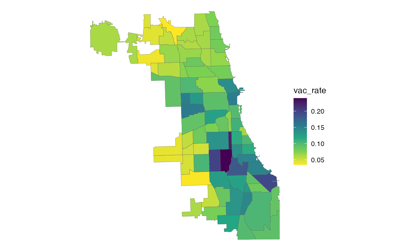
# Estimate CCA-level housing vacancy rates from block group-level Census data
df_blkgrp <- tidycensus::get_decennial(
  geography = "block group", variables = c("H1_001N", "H1_003N"),
  year = 2020, state = "IL", county = c("031", "043"), output = "wide"
) %>%
  suppressMessages() %>%  # Hide tidycensus messages
  select(geoid_blkgrp = GEOID, hu_tot = H1_001N, hu_vac = H1_003N)

df_cca <- xwalk_blockgroup2cca %>%
  left_join(df_blkgrp, by = "geoid_blkgrp") %>%
  mutate(hu_tot = hu_tot * hu_pct,
         hu_vac = hu_vac * hu_pct) %>%
  group_by(cca_num) %>%
  summarize_at(vars(hu_tot, hu_vac), sum) %>%
  mutate(vac_rate = hu_vac / hu_tot)
df_cca
#> # A tibble: 77 × 4
#>    cca_num hu_tot hu_vac vac_rate
#>      <int>  <dbl>  <dbl>    <dbl>
#>  1       1  28531  2129    0.0746
#>  2       2  28249  1756    0.0622
#>  3       3  35019  2804    0.0801
#>  4       4  20431  1288    0.0630
#>  5       5  15936  1005    0.0631
#>  6       6  61920  4199    0.0678
#>  7       7  38649  3079    0.0797
#>  8       8  77429 10744    0.139 
#>  9       9   4960   227    0.0458
#> 10      10  16035   704.   0.0439
#> # ℹ 67 more rows

# Join to cca_sf for mapping
library(ggplot2)
cca_sf %>%
  left_join(df_cca, by = "cca_num") %>%
  ggplot() +
    geom_sf(aes(fill = vac_rate), lwd = 0.1) +
    scale_fill_viridis_c(direction = -1) +
    theme_void()