Introduction

Activity-based models (ABMs) are founded on the idea that people’s travel behavior is a result of their daily activities; i.e., the things people need to accomplish dictate where, when, and how they travel, and with whom. These models are more advanced than standard travel demand models because they seek to represent the choices made by individual travelers. In order to do this, the models must generate a schedule of daily activities for members of every household in the region, and then transform that information into sequences of trips that occur throughout the day. To accomplish this, ABMs use detailed information about the factors that affect travel decisions, including:

  • Households – the number of adults, children, and workers; household income; the number of vehicles available
  • People – age; work and school status; occupation
  • Trips – purpose; destination; who is taking the trip; is it part of a sequence of trips that must be completed in a specific order
Having all of this data available for individual travelers allows for a finer level of analysis than standard travel demand models. ABMs were developed as a way to better analyze the impacts of policy decisions like managed lanes, congestion pricing and alternative transit fare structures. For more information, visit CMAP's Activity-Based Models.

CMAP's ABM platform is CT-RAMP (Coordinated Travel and Regional Activity-Based Modeling Platform), which was developed open source by a consultant under contract to CMAP. Activity-based modeling is increasingly viewed as a superior method to better understand the socioeconomic determinants of travel choice and for evaluating modern transportation solutions. CMAP's ABM has been developed to demonstrate sensitivity to highway pricing scenarios based on each traveler's individual value of time and to improve model sensitivity to a wider range of nontraditional transit attributes, i.e., attributes such as service reliability, personal safety, station and vehicle cleanliness, and crowding that do not typically inform transit Level of Service calculations. Subsequent work on the ABM has focused on the calibration of selected sub-models and the overall validation of the model results. This report represents the results of model calibration and validation activities completed over the last several years by CMAP staff and their consultants.


CMAP Modeling Area and Network


The modeling area extends beyond the 7-county CMAP region to include 21 counties. Only portions of Lee, Ogle, and LaSalle counties are included in the modeling area.


Model Steps

The following provides a brief outline of the major steps involved in running CMAP’s ABM. Preliminary sets of highway and transit trip assignments are run to generate realistic congested travel times that are used by CT-RAMP when daily activities are scheduled. The model also accounts for the relative ease or difficulty involved in reaching destinations using various modes of transportation, including driving, walking and using transit.


A synthetic population provides the foundation for modeling individuals’ travel behavior within an activity-based model. Using Census data and other socioeconomic information, a complete set of households for the CMAP modeling area is developed. (see Population Synthesis tab). This dataset contains all of the relevant attributes about each household and individual that are required by the ABM. Since the Census Bureau does not release detailed information about every household and individual, household and person records are replicated in order to generate a complete set of households for the modeling area. Target totals for various household and population attributes guide this process so the final population is representative of the region. All of the subsequent steps in the ABM rely on the data provided in the synthetic population.
Two sub-models are included in this step: one that models the usual workplace locations for workers and one that models the usual school location for students. The workplace location model accounts for the worker’s occupation, as identified by the industry category they are employed in within the synthetic person file. This information is paired with jobs within the employment categories summarized at a fine geographic level to ensure that workers are sent to locations where they could be employed in their field. Similarly, enrollment figures are provided for elementary schools, high schools and colleges to ensure students are sent to realistic school locations.
These models simulate four mobility attributes that affect individual transport mode decisions: 1) free parking eligibility for workers in the Central Business District, i.e., a determination of whether workers will pay to park; 2) household vehicle ownership; 3) whether or not individuals hold transit passes; and 4) whether or not individuals have toll transponders.
These models schedule activities and travel tours for all household members (see Tours tab). The first sub-model classifies daily travel patterns into three types:
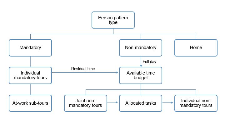
  • Mandatory (work and school) – includes at least one out of home mandatory activity;
  • Non-mandatory (other purposes) – includes at least one out of home non-mandatory activity but no out of home mandatory activities;
  • Home – in home activities only, so no travel is involved.

These activities are modeled as joint choices so that decisions made by household members affect the decisions of other members of the household. The next sub-models estimate the frequency and time of day for mandatory activities. These are given a higher priority for scheduling than non-mandatory and home activities. Following the scheduling of mandatory activities, individuals have “residual time windows” which can be used to schedule other activities including joint travel with other household members.

The next sub-model estimates joint travel for household members. All characteristics of joint travel (travel purpose, individual household members traveling, destination and time of day) are simulated. Joint travel is conditional upon the available time window for each household member following the scheduling of mandatory activities.

The next sub-model generates maintenance tours, which cover shopping and other household errands. These tasks are allocated to a single household member to carry out, and the destinations and times of day are generated. These tours are developed sequentially for individuals to ensure consistency in their personal schedule.

The next sub-model simulates discretionary tours which are modeled for individual, not joint, travel. These are also modeled sequentially so that they could all realistically occur during an individual’s day.

The final sub-model simulates at-work tours – those tours that occur during the day with the workplace as the starting and ending location.

These sub-models determine the transport mode used on tours, the locations of intermediate stops made on the tours and the purpose of each stop.
These sub-models add details about the trips occurring within the tours including the mode of travel, the departure time from each location and the parking location for auto trips. See Trip Mode tab and Trip Activities tab.
Following development of the complete set of daily activities, trips are assigned to the travel networks. Motor vehicle trips developed by the ABM are routed along the model transportation network from origin to destination in order to estimate traffic flows and network conditions. Transit trips are assigned to a network that includes all available bus and rail options between their origins and destinations. See Highway Assignment tab and Transit Assignment tab.


Population Synthesis

Using Census data and other socioeconomic information, a complete set of households for the CMAP modeling area is developed. This dataset contains all of the relevant attributes about each household and for each individual living in those households, which is required to run the ABM. While this population is statistically representative of the Census data, the actual households and individuals are “synthetic” in that they do not represent identifiable people and an individual household in the Census data may be replicated numerous times in order to generate a complete distribution of households in the modeling inputs.

The current population synthesis software used by CMAP is PopSynIII. The socioeconomic data developed from CMAP’s regional forecasting and Local Area Allocation procedures provide the subzone-level control values for all ON TO 2050 model scenarios. CMAP has greatly enhanced the functionality of PopSyn to enforce these controls and generate a distribution of enumerated households that account for the distribution of adults, workers and children within the agency’s forecasting procedures.

Individuals are classified into one of eight mutually exclusive categories:

  • Full-time worker: Age 16+ working at least 35 hours per week for more than 30 weeks out of the year.
  • Part-time worker: Age 16+ and a non-student employed less than full time.
  • Non-working adult: Age 16-64, non-working and a non-student.
  • Non-working senior: Age 65+, non-working and a non-student.
  • Pre-school: Age under 6.
  • Non-driving student: Age 6-15.
  • Driving age student: Age 16-19, not a full-time worker or college student.
  • University student: Age 18+ and school enrollment is college undergraduate or graduate school.
Data note: The observed data used Public Use Microdata Areas (PUMAs). PUMAs are statistical geographic areas defined by the U.S. Census Bureau for the dissemination of Public Use Microdata Sample (PUMS) data. Two of the PUMAs used to gather observed data include counties outside the CMAP modeling area (Stephenson County in Illinois, and Jefferson County in Wisconsin). Data for these PUMAs is weighted by the percentage of population or households – depending on the analysis – for counties within the CMAP modeling area. As a result, the total number of observed persons or households is not always identical for each summary analysis.

Population by Person Type

Note on "Full-time workers": The model defines full-time workers as persons working 30+ weeks in the year and 35+ hours per week. Full-time workers in the observed data are persons working 27+ weeks in the year and 35+ hours per week.


Hover over population categories to reveal details.


The model closely represents the number of full-time workers in the region (the largest person type by percentage). The model slightly overestimates the number of part-time workers and non-working adults. The largest disparities between the modeled and observed populations in terms of percentage points are for university students and non-working seniors. In both instances, the model is underrepresenting the population of these person types.


Households by Size


Hover over household size categories to reveal details.


In terms of the percentage of total households, the model slightly underrepresents one-person households in the region. The model also underrepresents the number of two-person households. However, three and four-person households are considerably overrepresented in the model. The largest disparity between modeled and observed households in terms of percentage is for large households (5+ people).

Household Characteristics

Households by


Income is in 1999 dollars.


The model does a reasonably well job of representing the various household characteristics. For instance, the number of 0-worker households is almost identical in the modeled and observed data, and the number of vehicles by household are very similar for modeled and observed households. The model slightly overestimates the number of lower income households and underestimates the number of high income households.


Household Detail

Distribution of Adults Per Household by


There is a discrepancy in the number of workers in households with one adult, and the model overestimates the total number of households with three adults. Similarly, when examining households by the number of children, the model overestimates the number of households with two adults and one child and underestimates the number of households with two children, regardless of the number of adults in the household.

Vehicle Ownership

Vehicle ownership plays an important role in individuals’ travel behavior decisions and helps define the set of travel mode options available to them. For example, households that own no vehicles may be dependent on transit to make their trips. Note that vehicle ownership refers to motor vehicles owned or leased by a household, including autos, pickup trucks, SUVs and motorcycles.


Number of Households by Vehicles Owned

Total Households: Model, Survey


The model does a good job predicting the number of vehicles owned by households. It is just slightly under-estimating the number of households with zero or 1 vehicle, and is just slightly over-estimating that number of households that own at least 2 vehicles.


Distribution of Vehicle Ownership by

Total Households: Model, Survey


Income is in 1999 dollars.


The model accurately predicts the distribution of vehicle ownership by household size, household income, and household workers. However, the model tends to under-estimate the number of households with at least 3 vehicles for larger households and high income households. It is also over-estimating the number of zero-worker households that own at least 2 vehicles.

Work Flows

Commute trips are an important part of a region’s overall travel pattern and are a key component of congestion experienced on the transportation system, especially during the morning and evening hours.  Ensuring that commuters are traveling between the appropriate home and work locations is one important way to verify that travel demand models reflect actual travel patterns.  

Note there are two sources for observed data on this page. The first three tables use data from journey-to-work flows from the Census Transportation Planning Package (CTPP). The remaining two charts use data from household travel surveys. CTPP data is generally used to estimate models that address work flows due to the large sample of data included. Data from household travel surveys can be used to supplement the journey-to-work information from the CTPP, as travel surveys offer more detailed information about the trips than the Census provides.


Modeled Journey to Work Flows


Observed Journey to Work Flows


Difference Model and Observed Journey to Work Flows


The model does a good job of replicating the number of commute trips being made within and between the counties in the CMAP region.  For instance, the model matches the Census data in showing that the top three work locations in northeastern Illinois are Cook, DuPage and Lake counties, in that order.  Both the modeled and observed data show that close to 45% of the total work trips made in the extended modeling area occur entirely within Cook County.  The model is underestimating the number of Cook and DuPage residents that live in one county and work in the other.  It is also underestimating the number of Cook residents that work in Lake and Will counties.


Origin and Destination Work Flows

From
To    


Hover over the chord diagram to see area boundaries on the map. Click on the map to see area name. Choose work flow geographies in the drop down menu to view numerical values for work trips.

Modeled


Observed


Work Trips by Mode and Distance


of all work trips


Shared ride 3+ toll and non-toll trips are combined due to the small sample of these trips captured by the Travel Tracker Survey.


Driving is the most frequently used mode for traveling to work in the region and the model does a reasonable job replicating the number of people driving different distances to work.  Nearly two-thirds of the commute trips in the region are people driving alone on trips that do not involve paying a toll and the modeled trips match the distance pattern for this group well, somewhat overestimating the extremely short trips (under 2.5 miles) and underestimating the trips longer than 30 miles.  A similar pattern is seen in the transit trips – the longer trips are underrepresented in the model and the shorter trips are overrepresented.

Trips by Mode

The CT-RAMP model includes eleven options for travel modes. These include the non-motorized options of walking or cycling, as well as transit, taxis and school bus. There are six options for auto trips, which are categorized by the number of vehicle occupants and whether or not the trip includes a toll. Vehicle occupancy categories include single occupants, two people sharing a vehicle, or more than two people sharing a vehicle.


Trips by Mode


See more about transit in the Transit tab.
Hover over bars to compare trips by mode.


While the model tends to overestimate walk trips, all other modes match observed trips fairly well. The model maintains relative shares among mode categories.

Trips by Person Type and Mode


of all trips

Individual trips only.


Modeled trip modes for non-student person types are close to observed trips modes. Though student trips are not reflected as accurately, they make up a small fraction of all trips. In many cases, modeled student trips are closer to the observed trips, in terms of number of trips, than other person types.

Trips by Household Income and Mode


of all trips


Income is in 2007 dollars.


The model overestimates lower income trips and underestimates higher income trips, but middle income trips compare well to the observed trips. For all household income categories, the mode trends are in agreement with the observed data.

Trips by Purpose and Mode


of all trips


See more about trip purpose in the Trip Activities tab.


Aside from a few, less impactful outliers such as transit and taxi trips for university activities, the model produces generally reasonable results for each trip purpose. The mode distributions of work and shop trips – the most common trip purposes and nearly half of all trips – have strong correlations to the observed trips.

Tours

Tours are chains of trips that start at one location and return to that same location. A common example is a trip made from home to work, followed by another commute trip returning home later in the day. Tours are composed of a minimum of two trips. Tours may also contain sub-tours, for example traveling from work to an external meeting and then returning to work. Tours may be completed by an individual or can include multiple people traveling together.

Daily activities are categorized into three types: mandatory, nonmandatory, or home. Activities are placed within these three categories based on the relative importance of the role they play in defining one’s day. Mandatory activities (which include work and school) are the most inflexible in terms of when they occur and where they are located. Nonmandatory activities have greater flexibility in when they occur and where their locations are. Home tours are stationary and are not assigned a travel mode.


Daily Activity Patterns By Person Type

of all tours


Bars show number of individual tours in the selected activity type (mandatory, nonmandatory) that will be scheduled for each person type. Activities that occur at home make up the remaining 16.3% of all tours, and these are not assigned a travel mode.


The model does a good job of matching the number of mandatory tours especially for full-time workers and non-driving students, which account for nearly 80% of mandatory tours. The modeled data also closely match the pattern of nonmandatory and home activities, with the notable exception being that the model is overestimating of the number of nonmandatory tours for non-working adults.

Tours by Person Type


Hover over bars to compare tours by person type.


The largest proportion of tours is for full-time workers, and the model slightly underrepresents these (3.89 million modeled tours vs. 4.05 million observed tours). Tours for part-time workers, non-working adults and non-working seniors are all noticeably overestimated by the model.

Tour Arrival and Departure Time of Day


Tour arrival and departure times are grouped into 40 time slices of the day.


Overall the model accurately predicts tour arrivals and departures by time of day, particularly for all trips.  Modeled work trips closely resemble observed work trips with noticeable peaks during the morning and afternoon/evening rush periods.  Modeled escort tours also resemble the observed data, though to a slightly lesser extent than more predictable work or school tours.  One tour type where the model differs from observed tours is university tours.  Whereas morning departure times are closely related, there is greater variability in the observed arrival times throughout the afternoon that the model does not necessarily capture.

Trip Activities

The CMAP ABM classifies trips into ten activity types. Activities can be grouped into two categories according to their priority in determining an individual’s schedule: mandatory and nonmandatory. Mandatory activities include:

  • Work - Working at regular workplace.
  • University - Attending college.
  • School - Attending school grades K-12.

The remaining activities are all considered nonmandatory:

  • Shopping - Shopping away from home.
  • Escort - Picking up/dropping off passengers (auto trips only).
  • Eating out - Eating outside of home.
  • Work-based - A subset of activities (such as going to lunch or traveling to meet a client) that occur with the place of work as the anchor location.
  • Maintenance - Activities that include medical appointments and other personal business or services that people engage in, excluding shopping and escorting activities.
  • Discretionary - Engaging in social or recreational activities; attending sporting or cultural events; and attending religious activities or performing volunteer activities.

Trip Activities


Hover over bars to compare trips by activity


The model overestimates work activities and underestimates maintenance and escort activities. The frequencies of all other activities are well represented. The difference in modeled and observed work activities could be related to the unusual economic conditions at the time the observed data was collected.

Trips by Person Type and Purpose


of all trips

Individual trips only.


With the exception of students under 16 years, the model does a better job matching observed non-student trip purposes. The one major difference among the non-student trips shows that the overestimation of work trip activities is limited to part-time workers.

Trips by Purpose and Distance


of all trips


The model is capable of capturing trip purposes for most trip distances, but tends to overestimate short trips and underestimate long trips. This behavior mostly applies to work trips.


Transit Trips

Transit is a vital part of the transportation system in northeastern Illinois and more than 600 million transit trips are made annually. It is important to properly calibrate such a key travel mode to ensure that the modeled transit trips reflect the travel sheds actually served by transit.


Modeled vs. Observed Transit Trips Origin and Destination

The scatterplot includes a point for each origin/destination pair. A map of origin/destination areas is shown below, with the CMAP region shaded for reference.

r2 =


The graph shows a strong correlation between the modeled and survey data.  The coefficient of determination (0.905) indicates the regression line is a good fit and accounts for more than 90% of the variation between the data sets.

Transit Trips by

Total transit trips: 1.63M Model, Survey
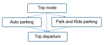

Distance is the distance of the transit trip that occurred. Income is in 2007 dollars. They survey has fewer total transit trips when viewed by income since not all respondents reported an income value.


The model overestimates the number of shorter transit trips (less than 10 miles) and underestimates the number of longer transit trips (greater than 15 miles). The greatest discrepancies are for very short trips (less than 2.5 miles) and very long trips (30 miles or more).

For transit trips by income, the model generally matches the observed data. However, the model significantly overestimates the number of transit trips made by persons in the $35k to $50k income range.

Transit Access

The Drive to Transit access mode includes individuals parking at transit stations (Park and Ride) and those who are dropped off at the station (Kiss and Ride).  The Walk to Transit access mode includes people walking or cycling to get to transit.


Hover over pie chart to compare transit access.
Modeled Transit Access

CMAP ABM - 2010 Scenario

Observed Transit Access

Travel Tracker Survey, 2007-2008


A slightly higher percentage of modeled transit trips (89.9%) are accessed by walking than observed transit trips (88.4%).

Synthetic Household Validation

This map displays the difference between modeled and observed data for selected household attributes summarized by U.S. Census Public Use Microdata Areas (PUMAs).  PUMAs are geographic areas defined by the U.S. Census Bureau that contain a minimum of 100,000 people.


Attribute: 0-vehicle households


Choose from household size, household income, number of workers, and number of vehicles in households by clicking the category button and selecting the specific household type from the dropdown. Hover over each PUMA to display the values for modeled and observed data.

Example: In the model, 22.7% of households in northeast Lake County are 1-person households. According to PUMS, 27.2% of households in northeast Lake County are 1-person households. This is a difference of -4.5 percentage points.


Highway Assignment

During Highway Assignment, the individual motor vehicle trips developed by the ABM are routed along the model transportation network from origin to destination in order to estimate traffic flows and network conditions.  As additional vehicles attempt to use the same roadway segments during the assignment, travel becomes more congested and travel times increase.  The assignment procedures implement a series of steps moving various portions of traffic onto alternative routes in an attempt to reduce congestion and minimize travel costs.  Equilibrium is reached within the highway assignment when vehicles cannot change paths without negatively impacting travel times.  Once equilibrium is reached, the volume of vehicles on each roadway segment is retained and can be used to calculate standard measures such as vehicle miles of travel (VMT).


Daily VMT Shares by County


In general, the model underestimates the total VMT for the 7-county region (160 million VMT vs. 167 million VMT). However, the VMT shares by county are very similar between the modeled and observed data. Counties with less VMT – like Kendall and McHenry – have very similar modeled vs. observed VMT shares, while Cook County accounts for 53.3% of modeled VMT and 50% of observed VMT.

Daily VMT Shares by County and Facility Type


The model does a good job of predicting the VMT shares by facility type for a few areas, including Suburban Cook and DuPage Counties.  The share of modeled vs observed VMT on local roads is almost identical for these two areas.  In Lake County, the model is overestimating the amount of VMT on interstates and underestimating the VMT on arterial streets.  In Chicago, the model is slightly underestimating the VMT on arterial streets.  In general, the share of modeled and observed VMT on arterials is lower in the City of Chicago, Suburban Cook County, DuPage County and Will County. 

Modeled vs. Observed Average Daily Link Volumes


r2 =


The scatterplot shows a strong correlation between the observed average daily link volume and the modeled daily link volume, which is verified with an r-squared value of 0.86. A value of 0.86 means that the regression line shown is a good fit of the observed data and accounts for 86% of the variation in the data. The correlation between the observed and modeled average daily link volumes is stronger for interstates than for arterials/collectors.

Daily VMT By Interstate

This comparison examines vehicles separated into two categories: auto (which includes cars, SUVs, pickup trucks, etc. that people drive for their personal use) and commercial vehicles (which include package delivery trucks all of the way up to tractor-trailers) used to conduct business activities.

Truck volumes on I-190 not shown due to bar scale. Model and observed values equals 11,512 and 9,917 respectively.


Hover over bars to display values and highlight segment on map. Click on a highway segment on the map to show the name.


Auto


Truck


The model over predicts the amount of weekday traffic on the interstate system. Separating the VMT into auto and commercial vehicle components shows that truck tollway freeway volumes are over estimated in the compared to the observed data. Overall, modeled auto volumes show a closer relationship to the observed data for both freeways and tollways.

Daily VMT by Volume Range


This analysis compares modeled volumes to links that have observed traffic counts on them.  Overall the model is overestimating traffic on these links by less than 2%, an extremely close margin.  VMT on the lowest volume roads are being overestimated, while VMT is underestimated by the model on the highest volume road segments.  For the five categories from 5,000 up to 59,999 the model is overestimating VMT by less than 9%, and for two categories the VMT difference is less than 2%.

Root Mean Squared Error Analysis


Links were grouped into volume bins based on the observed traffic counts (AADT) and linear regression analyses were completed for each group. The root mean squared error (RMSE) is a measure commonly-used for model validation analyses and compares the average difference between the observed values and the modeled volume predicted by the linear regression. The percent RMSE standardizes the value by dividing it by the average of the AADT. 

Target values represent the standard maximum acceptable root mean squared error from the Florida Department of Transportation, which are often cited as model validation goals.


For the lowest volume categories, which contain about 87% of the links measured, the percent RMSE is below the Florida target value. There is a spike in the 15,000-19,999 category, where the percent RMSE is 8 percentage points higher than the target value. The higher volume categories also exceed the target value but by smaller amounts. Overall this analysis shows that the ABM is dong a reasonable job of replicating the observed traffic counts.

Transit Assignment

The analysis of transit assignment results generally focus on comparing the number of transit boardings estimated by the model to observed boardings. The CMAP model transit network includes the following modes:

  • Heavy Rail – operated by the Chicago Transit Authority (CTA) in Chicago and some surrounding communities.
  • Commuter Rail – operated by Metra throughout the CMAP region.
  • Bus – operated by CTA (in Chicago and some surrounding communities) and by Pace Suburban Bus (in northeastern Illinois, mostly outside of Chicago).


Transit Boardings by Mode

Transit boardings include average weekday boardings for fixed-route service. Demand responsive dial-a-ride, call and ride, or ADA paratransit services are not included.


The model does a good job predicting the average number of weekday boardings for each transit mode. The predicted number of average weekday boardings for heavy rail, buses, and the total are very close to the observed data (all within 4%). The model is slightly underpredicting the number of transit boardings for commuter rail, by about 7%.

Transit Boardings by Line


Hover over bars to display values and highlight segment on map. Click on a transit segment on the map to show the name.

CTA


Metra


Overall, the model accurately estimates transit boardings by line for both CTA and Metra. The model overpredicts some of the transit boardings (such as the Green Line on the CTA and the BNSF line on Metra), while the model also underpredicts transit boardings on other lines (such as the Brown Line on the CTA and the MD-N line on Metra). However, for the most part, the model does a good job predicting the transit boardings on each CTA and Metra line.

Commute Trips Validation

The analysis of commute trips focuses on comparing the patterns of travel from home (place of residence) to work (primary place of work).


Modeled vs. Observed Journey to Work Flows

The scatterplot includes a point for each home/work county pair in the modeling area. Only a portion of Lee, Ogle, and LaSalle counties are included in the model data (refer to map in Introduction). A modeling area county map is shown below, with the standard CMAP region shaded for reference.

r2 =


The graph shows an extremely strong relationship between the data sets, which is verified by the value of 0.998. This coefficient of determination indicates that the regression line is a nearly perfect fit with the observed data and accounts for more than 99% of the variation in the data.


Modeled Journey to Work Flows


Observed Journey to Work Flows


Difference Model and Observed Journey to Work Flows


Almost half of the commute trips in the region originate from Cook County. Whereas the model does a good job of capturing the total commute trips originating from Cook County, it is overestimating the number of these trips that end in Cook County, and underestimating the number of commute trips from Cook to all other counties. The model is underrepresenting the total number of work trips originating from Lake County by 6.6%.